Mechanical Commutator vs Sensorless Commutation: How to Choose the Right Motor Commutation Method
We build commutators, so we see this decision from the part most discussions skip. Not “which motor type is newer.” That is not useful. The real question is whether your project needs a switching function built into the rotor, or whether it can afford to move commutation into the controller, the power stage, the startup logic, and the validation work that comes with that shift. Mechanical commutators still make sense when direct DC drive, simple reversing, low system cost, and fast transfer into production matter more than maximum efficiency or minimum maintenance. Brushless designs remove the brush-and-commutator interface, but they replace it with electronic commutation and a more demanding control stack.
That is why we do not treat brushed and brushless as a good-versus-bad argument. In many applications, either can work. The right answer usually comes from the total system: electronics budget, startup behavior, duty cycle, service interval, acoustic target, available design time, and how much variation the production line is expected to absorb without drama.
Table of Contents
What changes when a customer moves from mechanical to sensorless commutation
A mechanical commutator performs the switching physically. Brushes contact the commutator, current is routed into the rotor coils, torque follows. Sensorless BLDC removes that physical switching set. The motor still has to commutate, of course. It just does it electronically. In common six-step sensorless control, two phases conduct, one phase is left non-driven, and the controller watches the back-EMF behavior of that non-driven phase to decide the next switching instant. In steady operation, the commutation event is typically placed about 30 electrical degrees after the zero crossing.
On paper, that looks tidy. In a real product, it is not that tidy. The floating phase is only useful when it is actually readable. Right after commutation, switching transients and freewheel current can corrupt the sensing window. Reference implementations deal with this by delaying the point where back-EMF detection is allowed, skipping early samples, filtering the signal, or moving the sampling instant into a quieter part of the PWM cycle. So the engineering work does not disappear when the commutator disappears. It moves.
There is another practical point. At standstill, there is no useful back-EMF to read. So a sensorless BLDC drive does not really start “sensorlessly” from zero speed in the way many buyers assume. It usually needs an alignment step, a forced commutation ramp, or a startup state machine before the controller can hand over to back-EMF-based commutation. That handoff is one of the places where project schedules get longer than expected.
Why this matters to a commutator buyer
A buyer who starts with “brushless has no commutator, so it must be better” is usually looking at only one layer of the system. Sometimes that conclusion is right. Sometimes it creates new work in control electronics, EMC, startup robustness, or software validation that costs more than the mechanical wear problem they were trying to remove. Brushed motors remain attractive in many programs because commutation is built into the motor, control can be as simple as applied DC voltage or an H-bridge, and the architecture asks for fewer external elements.
We see this often in cost-sensitive products and in programs with short validation windows. If the application does not need the service-life advantage of a brushless platform, and if the noise, wear, and EMI of a brushed system are already manageable, a well-specified commutator is often the shorter route to production. Not more fashionable. Just shorter.
The selection screen we use early in a project
The table below is not a marketing comparison. It is the first engineering screen.
| Project condition | Mechanical commutator usually makes more sense | Sensorless commutation usually makes more sense |
|---|---|---|
| System cost ceiling is tight | Yes. Motor-side commutation reduces controller complexity. | Less often. Electronic commutation adds control hardware and validation. |
| Direct startup from rest matters | Strong fit. No back-EMF detection is needed to begin rotation. | Needs startup logic before back-EMF can be trusted. |
| Control architecture must stay simple | Strong fit. DC supply or basic H-bridge is often enough. | Weaker fit. Power stage and timing strategy are more involved. |
| Long maintenance interval is critical | Limited by brush and commutator wear. | Strong fit. No brush-and-commutator wear interface. |
| High-speed continuous duty is critical | Possible, but wear and thermal limits become more important. | Strong fit. Brushless designs are commonly chosen for long life at higher speeds. |
| Very low electrical noise and low arcing are required | More difficult. Brush contact and arcing must be managed carefully. | Usually better. No brush arcing at the commutation interface. |
| Production tolerance to electronics variation is low | Strong fit. Mechanical system is easier to standardize in many low-complexity products. | Weaker fit. Startup, sensing, and timing margins must be held in electronics and firmware. |
This tradeoff is consistent across mainstream motor references: brushed designs benefit from simpler control and fewer external components, while brushless designs trade that simplicity for longer life, higher-speed capability, and electronically managed commutation. Sensorless variants add another condition on top of that: startup and low-speed behavior have to be earned in control design, because usable back-EMF is a steady-running signal, not a standstill signal.
When we usually advise staying with a mechanical commutator
When the product needs straightforward DC operation, simple direction reversal, and fast ramp-up into production, mechanical commutation is still a very rational choice. It keeps the switching function inside the motor. That matters when the controller budget is small, the electronics team is not trying to build a motor-control platform from scratch, or the project simply does not want its main risk to move into software timing.
It also remains a practical choice when service intervals are understood and accepted. Brush wear is real. Commutator wear is real. But known wear, with known inspection intervals and known replacement rules, is often easier to manage than a redesign of the entire drive architecture. That is especially true in mature products where the mechanical envelope, power supply, and cost model are already fixed.
When sensorless BLDC is usually the better direction
When the project needs longer operating life without brush maintenance, sustained high speed, and lower losses at the commutation interface, brushless architecture starts to make more sense. That is the clean case. Remove the brush-and-commutator contact pair, move the windings to the stator, and the wear mechanism changes. So does thermal behavior. So does the service model.
But “sensorless” is not a free extra. It is usually the right path only when the application can tolerate startup logic, minimum-speed constraints, sensing-window design, and commutation timing work in exchange for removing position sensors. In steady running, back-EMF zero crossing is practical and widely used. At low speed and during launch, it is less forgiving. That distinction should be part of the cost discussion on day one, not week twenty-two.
If you keep a brushed platform, the commutator details decide whether it ships cleanly
This is where our factory work starts. A brushed motor does not succeed because the drawing says “commutator.” It succeeds because the commutation set is matched as a working system: commutator surface, brush grade, spring pressure, holder fit, and the thermal-current profile the motor will actually see in service. When those pieces are treated as separate purchasing lines, spark complaints tend to show up later. Usually in endurance tests. Sometimes in the field.
Surface condition is one of the first things we look at. A commutator surface cannot be too smooth and it cannot be too rough if the goal is stable current transfer and brush seating. Excessive mica height also creates trouble. So do burrs and poor bar-edge condition. These sound like small workshop details. They are not small once the brush film becomes unstable.
Brush matching comes next. The brush and the commutator are a pair, not two independent parts. Friction level, contact behavior, current distribution, and wear pattern all depend on that pairing. Spring pressure has to be high enough to maintain contact, but balanced across all brushes. Too little pressure and contact becomes unstable. Too much, and friction and wear go up. Holder clearance matters for the same reason: a brush that sticks or chatters cannot commutate cleanly for very long.
That is also why a commutator quote should never be based on diameter and segment count alone. Voltage, current, duty cycle, peak load, target life, brush material, rotational speed, and the actual switching profile all belong in the review. If those inputs are missing, the drawing may still look complete. The product will not be.
FAQ
Is a mechanical commutator still a reasonable choice for new motor programs?
Yes. In many applications, either brushed or brushless architecture can work. Mechanical commutation remains a good choice when the project values low system cost, simple control, fewer external components, and a faster path to production over the service-life and speed advantages of a brushless platform.
Does sensorless commutation always reduce total system cost?
No. It can reduce parts count by removing discrete position sensors, but it shifts work into startup logic, commutation timing, sampling strategy, power electronics, and validation. In projects where those development costs are significant, the total system cost may not improve as much as the motor-only comparison suggests.
Why do some BLDC programs still use Hall sensors instead of sensorless control?
Because sensorless back-EMF methods are strongest once the motor is already spinning and producing a usable signal. At zero speed and very low speed, startup has to rely on alignment, forced commutation, or another control strategy. Position sensors simplify that part of the operating range.
What usually shortens commutator life first?
Unstable brush contact, wrong brush pairing, poor surface condition, excessive mica, burrs, unequal spring pressure, and sustained sparking are common causes. These are not isolated defects. They interact. A surface problem often becomes a brush problem, then a wear problem, then an electrical-noise problem.
Can a brushed motor still be controlled with PWM?
Yes. One reason brushed motors remain useful is that speed control can be straightforward. Applied DC voltage changes speed over a wide range, and PWM with an H-bridge is a standard approach when variable speed or bidirectional motion is required.
What information do you need to review a custom commutator inquiry?
We usually start with rotor envelope, shaft speed, voltage, continuous and peak current, duty cycle, target life, brush material, available installation space, and the type of load. If the application already has brush wear or sparking data, that helps even more. It lets us tell quickly whether the fix belongs in the commutator design, the brush pairing, or the full commutation set.
Final note
The better choice is not the one with the better slogan. It is the one that matches the product architecture.
If your program needs a compact, proven, cost-controlled brushed solution, mechanical commutation is still a serious engineering answer. If your program has already crossed into long-life, high-speed, low-maintenance territory, then brushless electronic commutation may be the cleaner route. The mistake is not choosing one or the other. The mistake is comparing only the motor and ignoring the whole system around it.