6 Step Commutation BLDC: A Manufacturer’s View on Stable Switching
For BLDC systems, the commutator is no longer a copper part. It becomes switching order, timing margin, current path, and fault behavior.
That sounds obvious. On production lines, it is not.
Most 6 step commutation problems are not caused by the six steps themselves. They come from what sits around them: Hall placement drift, phase mismatch, weak startup strategy, noisy zero-crossing windows, uneven current decay, loose production control. The motor still turns. Then it gets hot. Or rough. Or inconsistent from lot to lot.
That is where we work.
When OEM customers discuss 6 step commutation BLDC designs with us, the conversation usually starts with speed and voltage. It should start earlier than that. With switching stability. With component matching. With how the commutator behaves when the sample leaves the bench and enters actual production.
Table of Contents
Why 6 step commutation is still widely used
Because it is practical.
For many industrial programs, 6 step commutation remains the preferred route when the target is straightforward drive architecture, predictable control cost, solid high-speed behavior, and manageable switching loss. It is not the smoothest method available. It does not need to be.
What matters is whether the system stays inside its stable operating window.
A clean 6 step BLDC platform should do four things well:
- start without hesitation under realistic load
- switch sectors without torque drop or current spike
- tolerate normal production variation
- remain debuggable when a field issue appears
If one of those is weak, the problem is rarely “BLDC theory.” It is usually commutator execution.
What we look at before approving a 6 step BLDC design
We do not begin with software language. We begin with the switching chain.
First, phase order.
Then Hall order.
Then the real commutation table.
Then PWM placement.
Then current waveform at each sector boundary.
Only after that do we discuss tuning.
This order matters. A wrong phase-Hall relationship can still spin the motor. That is why it wastes time. It creates a false pass condition during early testing, then becomes a noise or thermal issue later.
In other words, rotation alone proves very little.
The six-state sequence is simple. The production behavior is not.
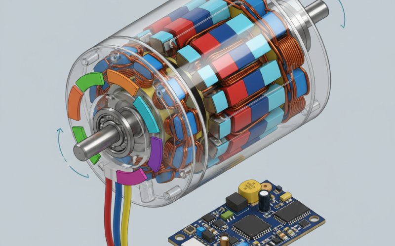
For a standard three-phase BLDC drive, each commutation step energizes two phases while one phase remains floating. That part is basic. The detail that matters more is what changes during each transition: current path, freewheel path, measurable voltage, and switching noise.
Here is the sequence structure we validate first for one rotation direction.
| Step | High-Side Phase | Low-Side Phase | Floating Phase | What We Check in Production |
|---|---|---|---|---|
| 1 | A+ | B- | C | Floating phase settles fast enough for valid sampling |
| 2 | A+ | C- | B | Sector change does not create current overshoot |
| 3 | B+ | C- | A | Hall edge or zero-cross point stays inside expected timing window |
| 4 | B+ | A- | C | Dead time does not distort torque delivery |
| 5 | C+ | A- | B | PWM still leaves a usable sensing window |
| 6 | C+ | B- | A | No illegal Hall state, no delayed commutation |
The table looks clean. Real motors are less polite.
A small Hall installation offset. Slight winding variation. A different cable harness. A tighter load at low temperature. Suddenly the same table does not sound the same anymore.
This is why we treat the commutation table as only the visible layer. The real product is underneath it.
Hall-based commutation: stable, but only when the map is real
Hall-based 6 step control is often presented as the easy version. Sometimes it is. Sometimes it only looks easy because the errors are hidden.
The common failure is not missing Hall sensors. It is incorrect mapping between Hall states and phase excitation. That mistake can survive prototype testing because the motor still rotates. Buyers see motion. Engineers hear roughness. Production sees return risk.
Our rule is strict here: Hall sequence must be confirmed against actual phase response, not assumed from motor wire color or naming convention.
We also treat illegal Hall states seriously. If 000 or 111 appears repeatedly in a standard three-Hall system, that is not cosmetic noise anymore. That is a reliability event. It usually points to sensor wiring, grounding, sensor placement, connector instability, or interface disturbance. A proper commutator design needs a fault response, not just a log entry.
Sensorless 6 step control: lower hardware count, higher startup discipline
Many OEM projects want sensorless control for cost, space, or harness reduction. Reasonable choice. But the startup logic has to be built with restraint.
At zero or very low speed, back-EMF is too weak to be trusted. So the motor must be brought up in open loop before the controller can hand over to zero-crossing based commutation. If that handover comes too early, the system may run on a light bench setup and still fail once inertia rises, grease thickens, or supply variation appears.
We see this often in sample reviews.
The issue is not that sensorless commutation is unreliable by nature. The issue is that many systems switch into closed-loop detection before the floating phase is truly readable. That creates random-looking field failures which are not random at all.
They were scheduled in at startup.
The floating phase is where weak designs reveal themselves
In sensorless 6 step BLDC control, the floating phase carries the information the commutator needs next. Which means it is also the phase most easily contaminated by poor timing decisions.
If the sampling window sits too close to PWM edge activity, the controller sees switching residue instead of usable back-EMF. Then the next commutation drifts. Then torque ripple increases. Then acoustic noise follows. Not always immediately. Enough to matter.
That is why we care about where the sample happens, not merely whether sampling exists.
A design that “supports sensorless” is not the same as a design with a robust zero-crossing window.
Torque ripple is not only a control problem
This point gets ignored too often.
Torque ripple in a 6 step BLDC system is influenced by control timing, yes. But in production it is also shaped by phase consistency, winding tolerance, rotor behavior, dead time setting, bus stability, and current decay during transitions.
So when a customer says, “the motor is rough,” the root cause may sit in firmware, inverter timing, or motor-side consistency. Treating it as a pure algorithm issue wastes debug cycles.
Our internal review usually checks three things together:
- commutation timing error
- current waveform distortion at sector boundaries
- component variation that pushes one batch closer to the limit than another
This is where supplier capability starts to matter. Not in slogans. In repeatability.
From mechanical commutator thinking to electronic commutator thinking
For teams moving from brushed platforms to BLDC platforms, the mindset shift is larger than expected.
A mechanical commutator is evaluated through material system, segment precision, insulation stability, wear path, brush contact behavior. An electronic commutator shifts the risk into phase logic, switching order, sensor interpretation, PWM timing, and protective action.
Different failure mode. Same commercial consequence.
That is why we do not separate the topic too sharply. For OEM programs, commutation is still a system question: how current is redirected, how timing is controlled, how the motor survives real duty, and how consistently the design can be reproduced across batches.
The hardware changed. The responsibility did not.
What a manufacturer should verify before shipment
For 6 step BLDC programs, we do not consider a design ready just because the motor reaches target speed.
We look for these release conditions instead:
1. Verified phase-Hall relationship
Not guessed. Not inherited from an old project. Verified.
2. Stable startup under actual load
No-load startup is not enough. Startup must be checked against the application’s real inertia and drag.
3. Controlled current at commutation boundaries
Current spike at each sector transition is one of the fastest ways to build heat and noise into the product.
4. Clean sensing window for zero-crossing detection
If the floating phase cannot be sampled repeatably, the control margin is smaller than the test result suggests.
5. Defined fault handling for illegal Hall states or missed commutation
A field-safe response should be part of the design, not a late patch.
6. Lot-to-lot consistency review
The commutator should survive normal manufacturing variation without being retuned for every batch.
Typical OEM mistakes we see with 6 step commutation BLDC projects
Some are small mistakes. They still cost time.
Treating the commutation table as universal
It is not. Motor lead order, Hall placement, and mechanical reference all matter.
Switching to sensorless feedback too early
Bench success at light load does not prove stable field startup.
Ignoring dead time as a torque quality factor
Dead time is often treated only as a safety setting. It also affects current shape and smoothness.
Measuring success by rotation only
A motor that spins can still be one tolerance shift away from production trouble.
Leaving the floating phase unreadable under PWM
Sensorless logic without a stable measurement window is only partly implemented.
When 6 step commutation is the right choice
We recommend 6 step BLDC architecture when the program values practical control cost, strong speed range, straightforward implementation, and proven manufacturability over ultra-smooth torque behavior.
That last part matters.
Not every customer needs the most advanced control method. Many need a design that starts, runs, scales, and ships without turning commissioning into a long software project. For those cases, a well-executed 6 step commutator is still the correct industrial answer.
Simple does not mean casual.
FAQ
What is the main benefit of 6 step commutation in BLDC motors?
The main benefit is control simplicity with solid industrial usability. It keeps the drive structure manageable while still delivering reliable operation across many OEM applications.
Why does a BLDC motor run on the bench but become unstable in production?
Because production exposes the margins. Load variation, Hall offset, harness difference, supply movement, and component tolerance all compress the commutation window. A bench test often hides that.
Is Hall-based commutation better than sensorless commutation?
Not universally. Hall-based control is usually stronger at startup and low speed. Sensorless control reduces sensor hardware and wiring. The correct choice depends on startup demand, cost target, packaging, and field environment.
Why is the floating phase important in sensorless BLDC control?
Because the controller reads back-EMF from the non-driven phase to estimate rotor position. If that signal is noisy or sampled at the wrong time, commutation accuracy falls quickly.
Can 6 step commutation meet OEM reliability requirements?
Yes, when phase mapping, startup logic, sensing window, transition current, and fault behavior are engineered as a complete system rather than treated as separate tasks.
What should buyers ask a supplier about 6 step BLDC commutation?
Ask how phase-Hall mapping is verified, how startup is validated under load, how commutation timing is checked in production, how illegal Hall states are handled, and how batch consistency is controlled.
Final Word
A 6 step commutation BLDC system does not become reliable because the six states are correct on paper. It becomes reliable when switching order, sensing, timing margin, and production control all agree with each other.
That is the difference between a motor that merely rotates and a platform that can be released to OEM production.